How to Cut TTS Latency for Real-Time Voice Apps: Practical, Measurable Steps

TL;DR — Key takeaways and recommended action plan

Cut latency fast with focused network, model, and pipeline fixes. For TTS latency optimization, start small: enable connection keepalives and TLS reuse, switch to streaming audio output, and pick a low-latency codec. Validate gains with simple bench tests that measure p50, p95, and p99.

Day 1 quick wins
1. Enable TCP keepalive and HTTP/2 or gRPC, reuse TLS sessions.
2. Test Opus or low-latency PCM, and enable streaming responses.
3. Run a 5-minute p95 latency test over your typical network.
Week 1 sprint
1. Add model-side streaming and chunked synthesis.
2. Reduce text preprocessing and batch sizes.
3. Run controlled A/B tests, collect p50/p95/p99 and Jitter.
Quarter plan
1. Deploy regional or edge inference, prewarm instances.
2. Re-architect buffering and adaptive jitter buffers.
3. Track cost versus latency, and set SLOs (service level objectives).

Quick validation checklist

Measure end-to-end time from request to first audio byte.
Compare streaming vs non-streaming under packet loss.
Automate nightly benchmarks to detect regressions.

Reduce latency, measure precisely, and iterate from quick wins to long-term infra changes.

Numbered 5-step infographic: Network, Model, Pipeline, Edge, Monitoring with one-line actions under each node.

What is TTS latency, and why does it matter for real-time synthesis

TTS latency optimization starts with understanding where time is lost. In live voice apps, latency adds up across capture, transport, processing, synthesis, and playback. This section defines each piece and explains how they shape the user experience.

Breakdown of delay sources

Microphone capture and pre-processing: Capturing audio includes ADC conversion and voice activity detection. If you use client-side noise suppression or echo cancellation, those add small delays.
Network transport: Packets travel to and from servers, and may queue at routers. Mobile and Wi-Fi links have variable jitter and can double the end-to-end delay.
STT and LLM processing: Speech-to-text (STT) or a large language model (LLM) may be used for intent or turn-taking logic. These compute stages can take tens to hundreds of milliseconds, depending on model size and batching.
TTS synthesis time: The TTS engine generates a waveform or vocoder output. Non-streaming synthesis blocks until complete, while streaming TTS emits audio progressively. Model complexity and token rate directly affect delay.
Audio pipeline and playback: Buffering, format conversion, and playback device latency matter. Many browsers and mobile players introduce 50 to 200 ms of buffering by default.

Human perception targets for conversational flow

<200 ms: ideal for audio feedback tied to immediate actions, like button clicks.
<500 ms: target for seamless turn-taking in dialogue, where users feel conversation is natural.
<1 s: acceptable for short system responses, though it may feel slightly slow.
1.5 s: likely to break the flow, causing users to interrupt or repeat themselves.

These targets guide tts latency optimization decisions and trade-offs between cost and responsiveness.

Common UX failure modes caused by high latency

Overlap: The system speaks while the user is still talking, causing interruptions and confusion.
Awkward gaps: Long silence makes the system feel slow or inattentive.
Repeated prompts: Timeouts cause retries, leading to duplicate audio or repeated instructions.

High latency damages trust and increases user friction. Reduce delays at each component for the best real-time synthesis experience.

How to measure latency: metrics, tooling, and benchmark methodology

Start by defining the exact numbers you will collect and why they matter for TTS latency optimization. Capture client-side, network, and server timings and keep traces linked across tiers. Below are the concrete metrics, how to tag traces, and a repeatable benchmarking plan you can run in CI and in production.

Core metrics to collect

Collect these metrics for every request and persist raw samples for percentiles:

Time-to-first-byte for audio (TTFB): time from request send to the first audio byte received.
First-audio-frame latency: time to the first playable audio frame decoded on the client.
End-to-end mouth-to-ear: from text input or play trigger to audible output start, includes TTS generation, transport, decode, and playback.
Jitter and packet loss: measure RTP/UDP jitter and packet loss per stream, and compute inter-arrival jitter.
p50, p95, p99, p999: report these percentiles for each metric and for combined mouth-to-ear.
Throughput and concurrency: requests per second, audio seconds generated per second, and CPU/GPU utilization.

How to tag traces across client, network, and server

Use a single trace ID propagated through headers and logs. Create spans for: client render, client buffer, network send, server receive, TTS synthesis, audio encode, and server transmit. Name spans consistently, for example: client. render, net send, server. synth, server.encode, net.recv. Capture key attributes: codec, sample rate, region, instance type, and network conditions (RTT, loss). Instrument both HTTP and WebRTC paths. For WebRTC stats, use the browser API to map RTP stream IDs to your trace ID.

Repeatable benchmarking methodology

Define test matrix: codec, sample rate, streaming vs non-streaming, regions, instance size.
Run warm-up runs to prime caches and models.
Execute steady runs at target load for 5 to 15 minutes, then burst runs with sudden spikes to observe tail behavior.
Collect at least 1,000 samples per cell for stable p99/p999 estimates.
Compare synthetic tests (controlled clients with network shaping like tc/netem) to production sampling (real clients via tracing and sampling).

Instrumentation and tooling

WebRTC internals: use the browser WebRTC stats API and about:webrtc logs. Note that Identifiers for WebRTC's Statistics API (2022) documents the totalProcessingDelay metric, which measures the sum of time each audio sample takes from RTP reception to decode. Use that metric to separate network vs processing delay.
Browser timing APIs: use PerformanceObserver and navigation/performance timing for rendering and decode events.
Prometheus and Grafana: export server and client metrics, create dashboards for p50/p95/p99/p999, and alert on p99 degradation. Follow official Prometheus exporter patterns for histogram buckets and labels.
Network tools: tc/netem for shaping, Wireshark/tcpdump for packet-level validation.

Run apples-to-apples comparisons by fixing codec, sample rate, and client buffer settings. Store raw traces and metric definitions in a repo so benchmarks are reproducible.

Try DupDub's low-latency TTS with a 3-day free trial

Network & transport optimizations for real-time synthesis

Network choices shape how fast you hear the first word and how smooth the audio stays. For TTS latency optimization, transport handshake, encryption work, and packetization rules combine to affect initial TTFB (time to first byte) and sustained frame latency. This section compares common transports and gives concrete, deployable fixes you can measure.

Pick the right transport: WebRTC, WebSocket, or HTTP/2

Which one you pick changes the tradeoffs for first-byte delay and steady-state frames. WebRTC uses UDP with ICE and DTLS, so its setup includes NAT traversal handshakes, but it yields low jitter and small packet sizes for steady audio. WebSocket uses TCP with an HTTP upgrade, so its handshake is lighter than a full TLS session but it relies on TCP ordering, which can add latency under packet loss. HTTP/2 has connection reuse and multiplexing, but TCP head-of-line blocking can hurt short audio frames.

Transport	Handshake cost	Encryption	Best for	Notes
WebRTC (UDP)	Medium-high	DTLS/SRTP	Lowest steady latency	ICE adds setup RTTs, but packets avoid TCP delays
WebSocket (TCP)	Low	TLS over TCP	Simple bidirectional streams	Use TCP_NODELAY and keepalives
HTTP/2 (TCP)	Medium	TLS over TCP	Multiplexed requests	Good for batching, worse for tiny frames

Concrete fixes you can apply today

Reduce hops and RTT: use anycast edge POPs and route optimization. Less network distance cuts TTFB.
Keep connections warm: TLS session resumption, HTTP/2 connection reuse, and WebSocket keepalives avoid repeated handshakes.
Use connection affinity: bind a client to an edge or regional instance so TURNovers and repeated ICE are rare. That also improves caching and CPU locality.
Tune transport-level settings: disable Nagle (TCP_NODELAY), enable TCP Fast Open where possible, and set aggressive keepalive intervals.
Optimize MTU and packetization: match UDP/TCP MTU to avoid fragmentation, and packetize short audio frames tightly to reduce per-packet serialization delay. Smaller frames lower codec buffering, but raise packet overhead. Test the tradeoff.
Prefer UDP-based stacks for sustained low jitter: when NAT traversal succeeds, UDP avoids head-of-line blocking and reduces frame latency.

Edge, CDN, and routing patterns

Place an edge POP near users, then route to a regional TTS service with affinity. Use CDN or edge routing that keeps TLS or QUIC connections open. If you must relay traffic, avoid TURN for every session; it adds an RTT. Measure each hop and prioritize changes that cut one or two RTTs.

Practical checklist: measure TTFB and per-frame RTT, compare transports under packet loss, and record CPU and network cost for each tuning. Small changes often yield the biggest wins.

Workflow diagram: client to edge POP to regional service to TTS engine, annotated with latency contributors; callouts for connection affinity and packetization tuning.

Model & inference optimizations (TTS engine, streaming vs non-streaming)

Reducing TTS latency optimization starts on the model path. Pick streaming when you need audio fast, and batch when you need top fidelity. This section shows practical rules, model levers, and provider knobs you can tune to drop tens to hundreds of milliseconds.

Streaming vs batch synthesis: rules of thumb

Streaming synthesis sends partial audio as tokens arrive. Use it for live chat, voice agents, or interactive assistants. Latency goes down because audio plays before the full sentence finishes. Tradeoffs: a small quality hit at word boundaries and extra buffering logic.

Batch (non-streaming) generates full audio before playback. Use it for long-form narration, one-off clips, or when you must apply heavy post-processing. It wins for peak perceptual quality, but adds end-to-end latency equal to generation plus encoding time.

When to pick which

Choose streaming if end-to-end lag must be under 200 ms for short replies.
Choose a batch for prerecorded content that can tolerate 500 ms or more.
Hybrid: stream smaller turns, batch long segments to save compute.

Model-side levers you can control

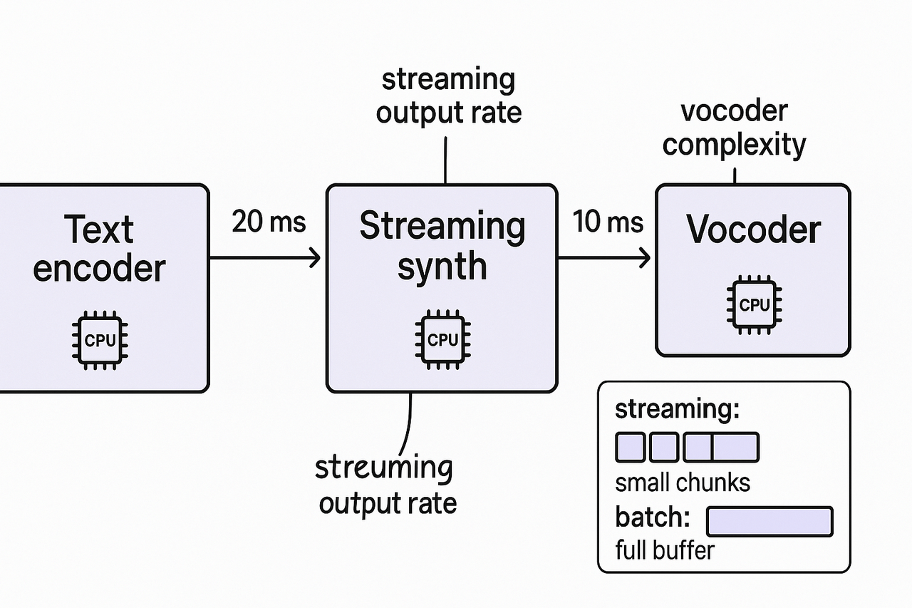
Model design and inference settings often offer the biggest wins. Tune these levers in priority order:

Model size: Smaller models reduce compute time and cold-start latency. Choose compact TTS for short utterances. Larger models improve nuance but add latency.
Pruning and quantization: remove redundant weights and use INT8 or dynamic quantization to cut CPU cycles. Perceptual quality often stays high.
Batching window: batch small concurrent requests for GPU throughput, but keep the window tight. A 10-50 ms window balances latency and efficiency.
Concurrency limits: cap simultaneous inferences to avoid queuing delays. Prefer autoscaling pools with short warmup.

Apply measured trade-offs. Start by halving model size or enabling int8 quantization, then re-benchmark.

Vocoder choice and provider knobs to shave latency

Vocoder complexity directly impacts final rendering time. Neural vocoders like HiFi-GAN give top quality but cost more time. Lightweight vocoders or hybrid Griffin-Lim style algorithms render faster with acceptable quality for many apps.

Provider-side knobs to tune on a DupDub-like API or third-party service:

Pick streaming endpoints with small chunk sizes.
Lower the sample rate to 22 kHz when 44.1 kHz is overkill.
Use low-latency vocoder presets if available.
Warm pools to avoid cold-starts and cache common phoneme outputs.
Reduce frame size and enable early audio flushing for partial plays.

Iterate with a repeatable benchmark. Measure per-component latency: encoder, streaming synth, and vocoder. Small changes add up, often saving tens to hundreds of milliseconds while keeping perceptual quality high.

Diagram showing Text encoder, Streaming synth, and Vocoder blocks annotated with streaming output rate and vocoder complexity.

Audio pipeline, buffering, and playback strategies

Start by treating audio buffering as a latency policy, not just a technical detail. For fast apps, TTS latency optimization begins at the smallest playable buffer you can reliably decode without glitches. Pick a baseline, measure perceived stutter, then iterate with adaptive buffers that react to jitter and CPU pressure.

Minimal viable buffer and adaptive jitter buffers

Aim for a minimal viable buffer of 40 to 120 ms of audio (client-side). That size gives the decoder a few frames for smooth playback while keeping per-utterance delay low. Use an adaptive jitter buffer (a small queue that grows or shrinks to absorb network variance) to add or drop 10–20 ms steps based on packet arrival patterns and decode timing. Monitor three signals and tune thresholds: packet inter-arrival variance, decode CPU load, and playback underruns. If you see repeated underruns, favor a slightly larger base buffer.

Chunking frames versus continuous streaming

Chunking frames gives you tight control over latency and CPU spikes. Continuous streaming reduces protocol overhead but can increase decoder CPU due to larger contiguous buffers. Trade-offs:

Chunked frames: send 20–40 ms frames. Benefit: quick playback start, easier partial-speech barge-in. Cost: more packets, slightly higher bandwidth overhead.
Continuous streaming: send a steady audio stream in larger blocks. Benefit: fewer context switches, lower packet overhead. Cost: longer time to first audible byte and heavier decoder work.

A pragmatic pattern: start with small chunks for the first 200–400 ms, then switch to larger blocks once steady-state playback is reached.

Client format, sample rate, and decoder cost

Choose OPUS for internet delivery when you need low bitrate and built-in packet loss resilience. Use PCM (WAV) when CPU decoding cost is the priority and the network is stable. Lower sample rates (16 kHz) cut bandwidth and CPU, but can harm voice naturalness. For voice-first apps, 24 kHz or 16 kHz is often the best compromise.

Partial-speech playback, barge-in, and turn-taking

Enable partial-speech playback so users hear audio as soon as the first frames arrive. Support barge-in by letting the client interrupt playback on an incoming user event, then fade or cut audio cleanly to avoid clicks. For handoffs, implement a soft turn-taking protocol: send a 30–100 ms silence marker before the speaker switch, confirm end-of-utterance tokens from the TTS engine, and apply a 10–50 ms overlap-tolerant crossfade to avoid truncation.

These patterns reduce perceived lag while keeping decoders and networks stable. They work across browser and native clients and scale to edge deployments where tight buffers matter most.

Edge deployments cut round-trip time by moving inference near users. For teams chasing TTS latency optimization, picking edge or regional hosting often yields the biggest win. This section compares trade-offs, shows where to place services for privacy, and lists minimal security hardening steps for voice-clone models and data protection.

Edge versus central-cloud: trade-off matrix

Use the table below to compare typical outcomes when you move TTS inference to the edge versus keeping it in a central cloud region.

Deployment	Latency reduction	Incremental cost	Operational complexity	Privacy/data residency
Single central region	Moderate	Low	Low	Moderate, depends on the region choice
Multi-region cloud	Good	Medium	Medium	Better, regional controls available
Edge on-prem / PoP	Best	High	High	Best, full data residency

The table shows patterns, not exact numbers. Aim for edge only when latency needs are below 100 ms, or when jitter kills UX.

Where to place services, and why it matters

Pick regions based on user density, not marketing. Start with your top three regions by peak concurrent users. For voice apps, prioritise locations that cut median RTT under 50 ms. For EU deployments, remember this rule: The General Data Protection Regulation (GDPR) prohibits restrictions on the free movement of personal data within the Union when based on reasons connected with the protection of personal data, as noted by European Commission Communication on Exchanging and Protecting Personal Data in a Globalised World (2017). That affects where you can replicate voice data for backups and model fine-tuning.

Quick placement checklist:

Place inference near the largest user cluster first.
Use multi-region fallback for failover and lower cold-starts.
Apply regional egress filters to limit cross-border copies.

Security hardening and privacy controls

Minimum controls for production voice cloning and TTS:

Model access control: role-based keys and short-lived tokens.
Encryption: TLS for transit and AES-256 for data at rest.
Key management: use KMS with audit logging.
Consent and retention: explicit user consent, retain minimal samples, and auto-delete after a retention window.
Audit and watermarking: log synthesis events and consider inaudible watermarks for cloned voices.

Cost note: edge lowers latency, but adds infra and ops cost. For most teams, hybrid deployments give the best cost-latency balance: run latency-critical inference at the edge, and batch or heavy training centrally.

Real-world case studies & benchmarks (anonymized)

Two anonymized production stories show practical wins from focused TTS latency optimization. Each case gives architecture notes, exact changes, and a brief benchmark table you can reproduce in your lab.

IVR: move from batch to streaming TTS

Background: A customer ran IVR prompts with on-demand batch synthesis. Calls stalled while the system waited for full audio files. We replaced full-file generation with streaming TTS over a persistent WebSocket (or HTTP/2) connection.

What changed: implement chunked audio frames, play partial buffers while synthesis continues, and prioritize hot prompts via an in-memory cache. Use short audio buffers (40–80 ms) and reduce codec framing overhead by using raw PCM or low-latency Opus. Co-locate TTS inference in the same region as telephony gateways.

Architecture notes:

Persistent stream between app and TTS engine (WebSocket/HTTP2).
Small jitter buffer in the client to smooth network variability.
Warm pools of model workers to avoid cold starts.

Benchmark summary (interaction-level):

Metric	Before	After
p50 interaction latency	400 ms	80 ms
p95 interaction latency	1,200 ms	220 ms

Repro steps: run 10 concurrent calls, send 1 short prompt per call, measure time-to-first-audio and time-to-complete, repeat cold and warm worker scenarios.

Multilingual dubbing pipeline: quality vs speed

Background: a media team needed fast localization with voice cloning similar to DupDub. They needed a repeatable balance of fidelity and throughput.

What changed: pre-generate cloned voice embeddings, batch sentences into 8–12 second chunks, and use a streaming vocoder for early playback. For final export, run a high-quality pass if time allows.